Introduction
The menzerath package is used to describe fit and plot data following the Menzerath’s law. Menzerath’s law (also known as Menzerath-Altmann law) was initially formulated as a linguistic law describing the relationship between the size of a linguistic construct and its constituents. Consider for example the relationship between the size of a word (y) and its syllables (x). According to Menzerath’s law in its standard formulation the expected relationship should follow:
y = a ⋅ xb ⋅ e − *c**x* where a, b and c are parameters of the law.
Installation
The package can be installed from github in R by running the following commands:
install.packages("devtools")
devtools::install_github("sellisd/menzerath", build_vignettes=TRUE)
the build_vignettes=TRUE can be omitted but then the vignettes will not be installed.
Usage
Basic Usage
To demonstrate how to use the package we are going to analyze a classic dataset originally used by Altman 1980 in the mathematical formulation of the Menzerath-Altmann law. The dataset relates the word size, measured in terms of number of syllables to the average syllable size in the word. The size of syllables is measured in terms of number of phonemes.
First we load the library and have a look at the dataset
library(tidyverse)
#> ── Attaching packages ─────────────────────────────────────── tidyverse 1.3.0 ──
#> ✓ ggplot2 3.3.3     ✓ purrr   0.3.4
#> ✓ tibble  3.1.0     ✓ dplyr   1.0.4
#> ✓ tidyr   1.1.2     ✓ stringr 1.4.0
#> ✓ readr   1.4.0     ✓ forcats 0.5.1
#> ── Conflicts ────────────────────────────────────────── tidyverse_conflicts() ──
#> x dplyr::filter() masks stats::filter()
#> x dplyr::lag()    masks stats::lag()
library(menzerath)
data(morpheme_syllable)
morpheme_syllable
#> # A tibble: 5 x 2
#>       x     y
#>   <dbl> <dbl>
#> 1     1  3.1
#> 2     2  2.53
#> 3     3  2.29
#> 4     4  2.12
#> 5     5  2.09
We can transform the table to a menzerath object and create a plot:
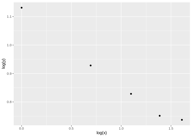
Then estimate the parameters of the law:
fit_menzerath <- fit(ms)
print(fit_menzerath)
#>
#> Call:
#> lm(formula = log(object$y) ~ log(object$x) + object$x, data = as.data.frame(x = object$x,
#>     y = object$y, stringsAsFactors = FALSE))
#>
#> Coefficients:
#>   (Intercept)  log(object$x)       object$x
#>       1.08529       -0.36854        0.04764
As a linear fit is performed on log scale in order to get the estimated parameters the coefficients have to be transformed. This is facilitated by the get_parameters function:
get_parameters(fit_menzerath)
#> $a
#> [1] 2.9603
#>
#> $b
#> [1] -0.3685362
#>
#> $c
#> [1] -0.04764427
The fit can also be visualized with a ribbon plot:
plot(ms, fit=TRUE)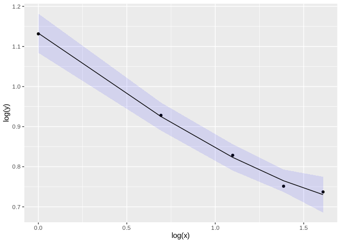 We can now repeat the same analysis in a more recent and larger dataset (Torre et al., 2019). The
 BG_word_time dataset contains the relationship between the size of breath groups and average word size (in seconds). Breath groups are defined by pauses (e.g. for breathing) during speech.
BG_word_time
#> # A tibble: 45,034 x 2
#>        x     y
#>    <dbl> <dbl>
#>  1     1 0.405
#>  2     1 0.329
#>  3     1 0.146
#>  4     9 0.318
#>  5    10 0.223
#>  6     1 0.442
#>  7     4 0.323
#>  8    11 0.213
#>  9     1 0.261
#> 10     7 0.309
#> # … with 45,024 more rows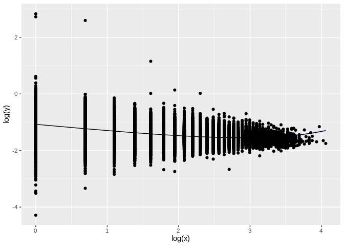
Alternative models
Different mathematical formulations of Menzerath’s law have been proposed.
| method name | equation | parameters | reference |
|---|---|---|---|
| simplified_1 | y = ae − cx | a, c | Altmann 1980 |
| simplified_2 | y = *a**xb* | a, b | Altmann 1980 |
| MAL | y = axbe − cx | a, b, c | Altmann 1980 |
| Milicka_1 | Ln − 1 = anLn − bnecnLn | an, bn, cn | Milicka 2014 |
| Milicka_2 | Ln − 1 = anLn − bn | an, bn | Milicka 2014 |
| Milicka_4 | $L\_{n-1} = a\_n + \\frac{b\_n}{L\_n}$ | an, bn | Milicka 2014 |
| Milicka_8 | $L\_{n-1} = a\_n + \\frac{b\_n}{L\_n} + \\frac{c\_n\\min(1,L\_n-1)}{L\_n}$ | an, bn, cn | Milicka 2014 |
Note that methods Milicka_1 and Milicka_2 are identical to the classical Menzerath-Altman formulation (MAL) and simplified_2 correspondingly. The only difference besides notation is the parameter sign so b = − bn and c = − cn.
In the classic example of syllable length of Indonesian morphemes Altman estimated a = 2.9603, b = -0.36853 and c = 0.04764. Using the same parameter estimates we can draw the expected form of the law with the different methods.
morpheme_length_vector <- c(1,2,3,4,5)
parameters = c(a=2.9603, b=-0.36853, c=0.04764)
menzerath_methods <- c("simplified_1", "simplified_2", "MAL", "Milicka_1", "Milicka_2", "Milicka_4", "Milicka_8")

mean_syllable_length_vector <- numeric(0)
for(i in c(1:length(menzerath_methods))){
  mean_syllable_length_vector <- c(mean_syllable_length_vector, dmenzerath(morpheme_length_vector,parameters=parameters, method=menzerath_methods[i]))
}
tibble(method = rep(menzerath_methods, times=rep(length(morpheme_length_vector),length(menzerath_methods))),
       morpheme_length = rep(morpheme_length_vector, length(menzerath_methods)),
       mean_syllable_length = mean_syllable_length_vector) %>%
ggplot(aes(x=morpheme_length, y = mean_syllable_length, color = method)) + geom_line()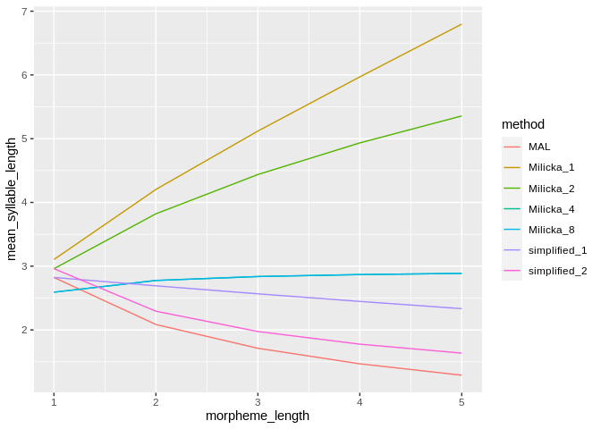
More interesting is to use these alternative models to estimate the parameters from real data. We can do so using Altmann’s data (Altman 1980) on syllable length of indonesian morphemes:
library(cowplot)
ms <- menzerath(morpheme_syllable)
MAL_plot <- plot(ms, fit=TRUE, method="MAL") + ggtitle("MAL")
simplified_1_plot <- plot(ms, fit=TRUE, method="simplified_1") + ggtitle("simplified_1")
simplified_2_plot <- plot(ms, fit=TRUE, method="simplified_2") + ggtitle("simplified_2")
Milicka_1_plot <- plot(ms, fit=TRUE, method="Milicka_1") + ggtitle("Milicka_1")
Milicka_2_plot <- plot(ms, fit=TRUE, method="Milicka_2") + ggtitle("Milicka_2")
plot_grid(MAL_plot, simplified_1_plot, simplified_2_plot ,Milicka_1_plot, Milicka_2_plot, ncol = 3)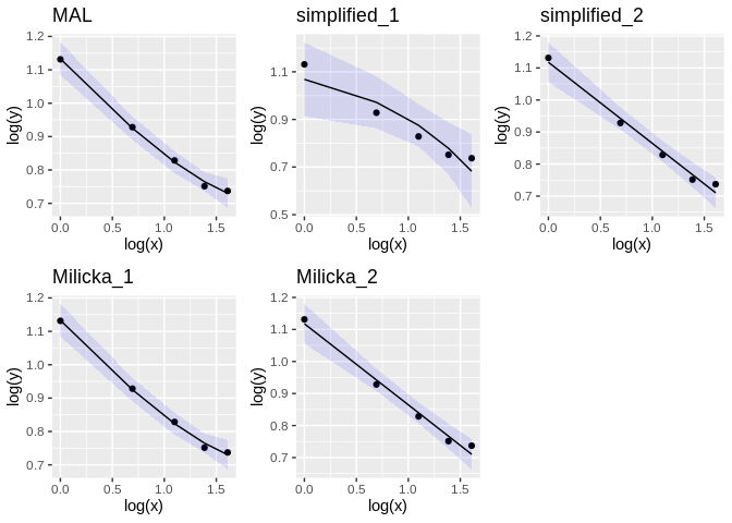
Datasets
In the menzerath package a number of datasets are included in the form of tibbles that can easily be loaded and manipulated to serve as examples or test data. There are some classic datasets from Altmann 1980 and some more recent ones from Torre et al. 2019
Datasets in package
-
morpheme_syllable: Dataset from Altmann 1980 linking morpheme size and syllable size. -
word_syllable_phoneme: Dataset from Altman 1980 on syllable length in English words. -
word_syllable_time: Dataset from Altman 1980 on syllable length in Bachka-German words. -
BG_word_characters: Dataset from Torre et al. 2019 linking breadth group size and average word size (in number of characters). -
BG_word_phonemes: Dataset from Torre et al. 2019 linking breadth group and average word size (in phonemes). -
BG_word_time: Dataset from Torre et al. 2019 linking breadth group and word size (in seconds).
Further documentation and details about each dataset can be gained with the help command, e.g:
help(morpheme_syllable)References
Altmann, G., 1980. Prolegomena to Menzerath’s law. Glottometrika, 2(2), pp.1-10.
Torre Iván G., Luque Bartolo, Lacasa Lucas, Kello Christopher T. and Hernández-Fernández Antoni 2019 On the physical origin of linguistic laws and lognormality in speech R. Soc. open sci.6191023 http://doi.org/10.1098/rsos.191023
Milička, Jiří. (2014). Menzerath’s Law: The Whole is Greater than the Sum of its Parts. Journal of Quantitative Linguistics. 21. 10.1080/09296174.2014.882187.
Contributing
Please note that this package is released with a Contributor Code of Conduct. By contributing to this project, you agree to abide by its terms.
